User Guide
SCEC Community Models Viewer Overview
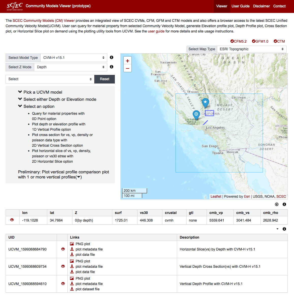
The CM Viewer provides a map-based access to UCVM version 19.4 release. It allows users to retrieve material properties from different Community Velocity Models. It also allows user to create 1D vertical profiles, 2D vertical cross sections and 2D horizontal slices from retrieved material properties
The pages on this site are the CM viewer page, this user guide, a disclaimer, and a contact information page.
The main interface is on the Viewer Page. On top of the map, there are selection buttons for overlay to include fault information from CFM, geological regions from GFM and/or heat flow regions from CTM.
Also on top of the map, there is a control that allows the base map to be changed. By default, the map shown is ESRI Topographic. The other map types are: ESRI National Geographic, ESRI Imagery, OTM Topographic, and OSM Street.
Both material properties and downloadable results are populated into two tables at the bottom of the interface page. Click on the eye icon () to highlight related location on the map. To return to non map select mode, return the selection dropdown to 'Select' mode. To return to the initial view, click the "RESET" button.
Model Selection
A subset of UCVM models are deployed and selectable in the viewer. The boundary of the selected model is displayed on the map. For model details please refer to the UCVM documentation--here.
Z Mode Selection
There are two query modes to select from: by elevation or by depth. Query by elevation is for Z in meters above or below the sea level. An elevation of -100 meter is 100 meter below the sea level and elevation of 200 meter is 200 meter above the sea level. Query by depth is for Z in meters at or below the surface. A depth of 0 is at the surface and a depth of 1000 meter is 1000 meter below the surface.
Material Property Search
When performing material property search, there are two location selection methods. The first method is to enter the latitude/longitude values of the location into the text boxes, then clicking the search icon (). The second method is to pick a point on the map with a mouse click. The text boxes will be populated with values from the selection. Next, initiate the search by clicking the search icon (). User can also select a local file to upload composed of latlongs and Z values. Remember to select the right Z mode for the Z values in the file.
1D Vertical Profile
Plotting of the depth or elevation vertical profile also uses the same location selection methods used by the material property search. The Z step is the vertical step in meters.
2D Vertical Cross Section
Plotting of a vertical cross section requires drawing a line on the map by either entering into the text boxes or by clicking a starting and an ending locations on the map. Default starting Z, ending Z and data type can be adjusted to different values.
2D Horizontal Slice
Plotting of a horizontal slice requires drawing a rectangle on th map by either entering into the text boxes or drag and draw a rectangle on the map. Default Z and data type can be adjusted to different values.
To return to the initial view with no selection, click the "RESET" button.
Browser Requirements
This site supports the latest versions of Firefox, Chrome, Safari, and Microsoft Edge.
About the SCEC Unified Community Velocity Model (UCVM)
More information about the UCVM can be found at: https://www.scec.org/research/ucvm
Overview
- Small, P., Gill, D., Maechling, P. J., Taborda, R., Callaghan, S., Jordan, T. H., Ely, G. P., Olsen, K. B., & Goulet, C. A., (2017). The SCEC Unified Community Velocity Model Software Framework. Seismological Research Letters, 88(5). doi:10.1785/0220170082. SCEC Contribution 2067
Models
- J. H. Shaw, A. Plesch, C. Tape, M. P. Suess, T. H. Jordan, G. Ely, E. Hauksson, J. Tromp, T. Tanimoto, R. Graves., K. Olsen, C. Nicholson, P. J. Maechling, C. Rivero, P. Lovely, C. M. Brankman, J. Munster (2015). Unified Structural Representation of the southern California crust and upper mantle. Earth and Planetary Science Letters. 415 1, doi: 10.1016/j.epsl.2015.01.016 SCEC Contribution 2004
- Lee, E.-J., P. Chen, T. H. Jordan, P. J. Maechling, M. A. M. Denolle, and G. C. Beroza (2014), Full 3-D tomography for crustal structure in Southern California based on the scattering-integral and the adjoint-wavefield methods, J. Geophys. Res. Solid Earth, 119, doi:10.1002/2014JB011346. SCEC Contribution 6039
- Lin, G., C. H. Thurber, H. Zhang, E. Hauksson, P. Shearer, F. Waldhauser, T. M. Brocher, and J. Hardebeck (2010), A California statewide three-dimensional seismic velocity model from both absolute and differential times. Bulletin of the Seismological Society of America, 100, 225-240. doi: 10.1785/0120090028. SCEC Contribution 1360 SCEC Contribution 1360
- Ely, G., T. H. Jordan, P. Small, P. J. Maechling, (2010), A Vs30-derived Near-surface Seismic Velocity Model Abstract S51A-1907, presented at 2010 Fall Meeting, AGU, San Francisco, Calif., 13-17 Dec.
- Pitarka, A., and Graves, R. (2010). Broadband Ground-Motion Simulation Using a Hybrid Approach. Bulletin of the Seismological Society of America, Vol. 100, No. 5A, pp. 2095–2123, doi: 10.1785/0120100057.
- Wald, D. J., and T. I. Allen (2007), Topographic slope as a proxy for seismic site conditions and amplification, Bull. Seism. Soc. Am., 97 (5), 1379-1395, doi:10.1785/0120060267. Wills, C. J., and K. B. Clahan (2006), Developing a map of geologically defined site-condition categories for California, Bull. Seism. Soc. Am., 96 (4A), 1483-1501, doi:10.1785/0120050179.
- Kohler, M., H. Magistrale, and R. Clayton (2003). Mantle heterogeneities and the SCEC three-dimensional seismic velocity model version 3, Bulletin Seismological Society of America 93, 757-774. SCEC Contribution 630